前言

QuTip是用于模擬開放量子系統(tǒng)動力學(xué)的開源庫。QuTip庫依賴于的Numpy、Scipy和Cython的數(shù)值包。此外,matplotlib提供了圖形輸出。http://qutip.org/。

python安裝比較容易，需要選擇一個版本，python2或python3，稍微麻煩的是Scipy。

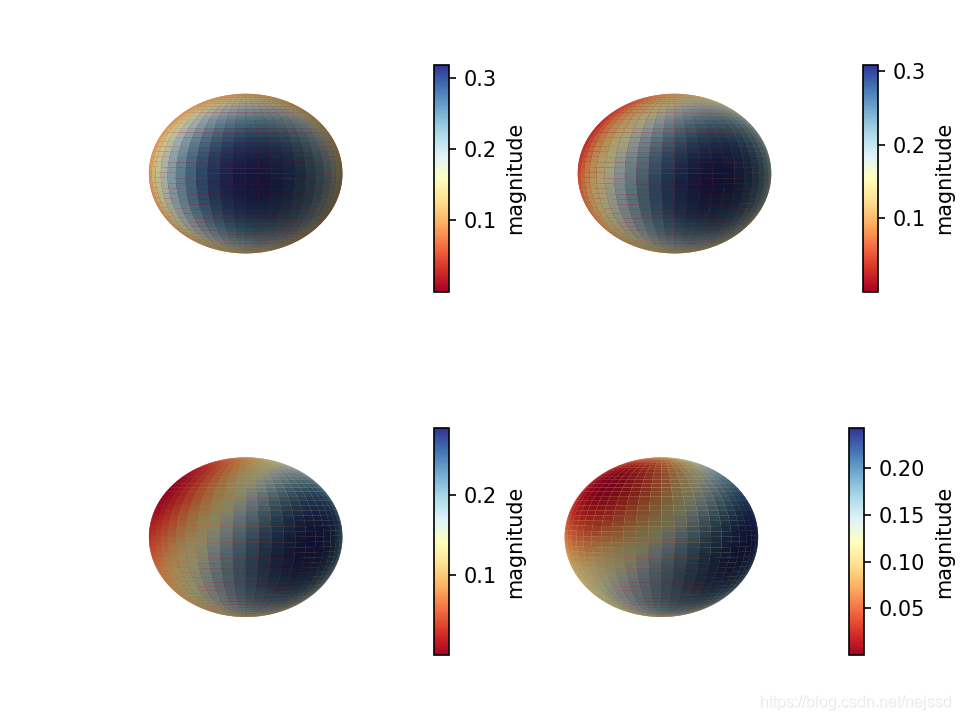
一、N原子系綜自旋概率分布

from qutip import *import numpy as npimport matplotlib.pyplot as pltn=2#原子數(shù)j = n//2psi0 = spin_coherent(j, np.pi/3, 0)#設(shè)置系統(tǒng)的初態(tài)為自旋相干態(tài)Jp=destroy(2*j+1).dag()#升算符J_=destroy(2*j+1)#降算符Jz=(Jp*J_-J_*Jp)/2#JzH=Jz**2#系統(tǒng)的哈密頓量tlist=np.linspace(0,3,100)#時間列表result=mesolve(H,psi0,tlist)#態(tài)隨時間的演化theta=np.linspace(0, np.pi, 50)phi=np.linspace(0, 2*np.pi, 50)#分別計算四個狀態(tài)下的 husimi q函數(shù)Q1, THETA1, PHI1 = spin_q_function(result.states[0], theta, phi)Q2, THETA2, PHI2 = spin_q_function(result.states[30], theta, phi)Q3, THETA3, PHI3 = spin_q_function(result.states[60], theta, phi)Q4, THETA4, PHI4 = spin_q_function(result.states[90], theta, phi)#在四個子圖中分別畫出四個狀態(tài)下的husimi q函數(shù)fig = plt.figure(dpi=150,constrained_layout=1)ax1 = fig.add_subplot(221,projection=’3d’)ax2 = fig.add_subplot(222,projection=’3d’)ax3 = fig.add_subplot(223,projection=’3d’)ax4 = fig.add_subplot(224,projection=’3d’)plot_spin_distribution_3d(Q1, THETA1, PHI1,fig=fig,ax=ax1)plot_spin_distribution_3d(Q2, THETA2, PHI2,fig=fig,ax=ax2)plot_spin_distribution_3d(Q3, THETA3, PHI3,fig=fig,ax=ax3)plot_spin_distribution_3d(Q4, THETA4, PHI4,fig=fig,ax=ax4)for ax in [ax1,ax2,ax3,ax4]: ax.view_init(0.5*np.pi, 0) ax.axis(’off’)#不顯示坐標(biāo)軸fig.show()

運行結(jié)果：

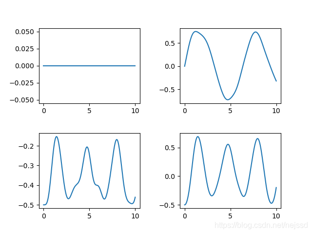
二、原子與光場相互作用

from qutip import *import numpy as npimport matplotlib.pyplot as pltalpha=1#相干光的參數(shù)alphan=2#原子數(shù)j = n/2psi0 = tensor(coherent(10,alpha),spin_coherent(j, 0, 0))#設(shè)置系統(tǒng)的初態(tài)a=destroy(10)#光場的湮滅算符a_plus=a.dag()#光場的產(chǎn)生算符Jp=destroy(n+1).dag()#原子的升算符J_=destroy(n+1)#原子的降算符Jx=(Jp+J_)/2#原子的Jx算符Jy=(Jp-J_)/(2j)#原子的Jy算符,這里的j是虛數(shù)單位Jz=(Jp*J_-J_*Jp)/2#原子的Jz算符H=tensor(a,Jp)+tensor(a_plus,J_)#系統(tǒng)的哈密頓量tlist=np.linspace(0,10,1000)#時間列表result=mesolve(H,psi0,tlist)#態(tài)隨時間的演化fig=plt.figure()ax1 = fig.add_subplot(221)ax2 = fig.add_subplot(222)ax3 = fig.add_subplot(223)ax4 = fig.add_subplot(224)ax1.plot(tlist,expect(tensor(qeye(10),Jx),result.states))#Jx的平均值隨時間變化圖ax2.plot(tlist,expect(tensor(qeye(10),Jy),result.states))#Jy的平均值隨時間變化圖ax3.plot(tlist,expect(tensor(qeye(10),Jz),result.states))#Jz的平均值隨時間變化圖ax4.plot(tlist,expect(tensor(qeye(10),Jx**2+Jy**2+Jz*2),result.states))#J平方的平均值隨時間變化圖fig.subplots_adjust(top=None,bottom=None,left=None,right=None,wspace=0.4,hspace=0.4)#設(shè)置子圖間距fig.show()

運行結(jié)果：

總結(jié)

到此這篇關(guān)于Python中qutip用法的文章就介紹到這了,更多相關(guān)Python qutip用法內(nèi)容請搜索好吧啦網(wǎng)以前的文章或繼續(xù)瀏覽下面的相關(guān)文章希望大家以后多多支持好吧啦網(wǎng)！